How do you get a bimodal distribution from a uniform distribution function?

Given a uniformly distributed random-number-generating function, f(), how can you transform it into a function with a bimodal distribution, g()?

A histogram of a normal distribution. Randomly sampled values are evenly weighted across the output range.

A bimodal distribution. Most values (mode) clump in two (bi) heaps, hence "bimodal".

This is the question that I dealt with as I overengineered my blog. I wanted to tilt my posts, to give the effect of papers loosely placed on a desk.

a few angled posts

I didn't want a normal distribution of post angles. Having the average post angle upright seemed boring. Rather, I wanted a bimodal distribution. This would have most posts angled slightly left or slightly right, with a few posts angled upright. I felt this would have a nice contrast between left and right angled posts, while still having natural variety.

Armed with Math.random() as my uniformly-distributed random function, I set off to figure out how to transform it into a bimodally-distributed random function.

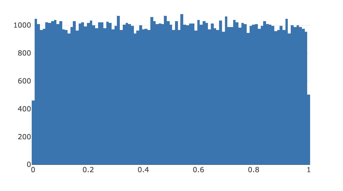
A histogram chart of Math.random() samples.

Simple transform functions

Just to understand what some common transforms might look like, I tried plotting them out.

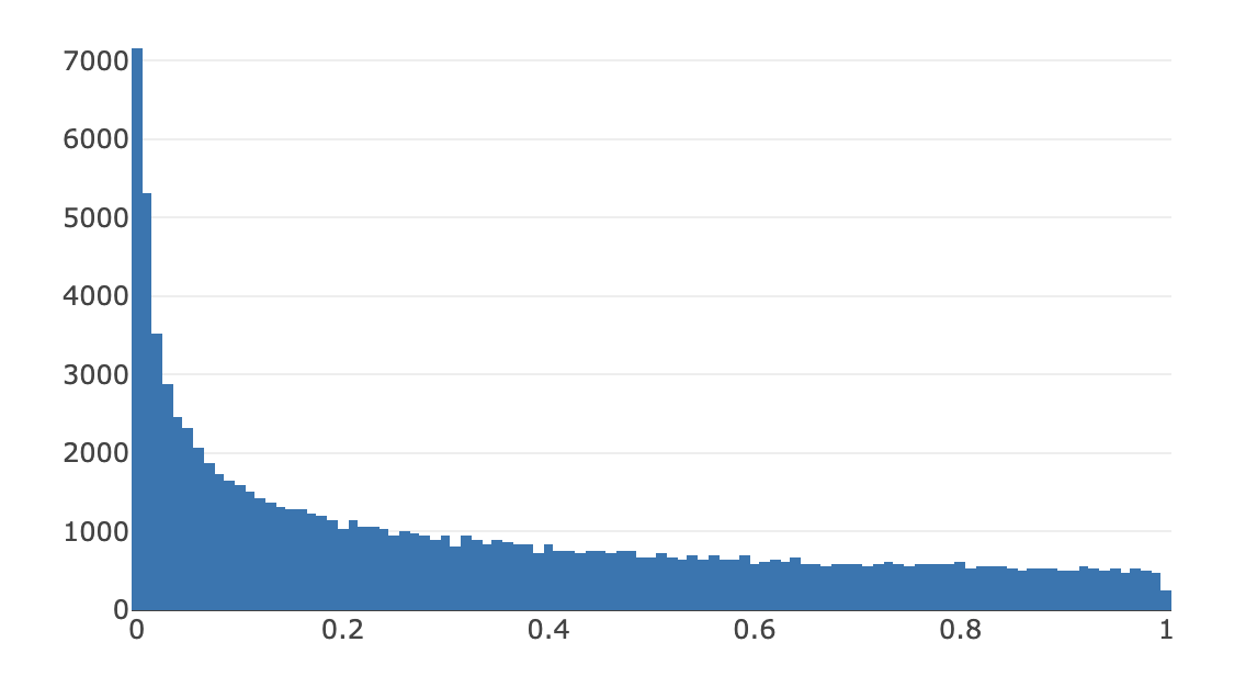
This histogram, which comes from plotting Math.pow(Math.random(), 2) samples, looks like a power law distribution:

(About half of the total samples in this distribution are less than 0.25.)

The distribution of these Math.sqrt(Math.random()) samples feels fairly linear:

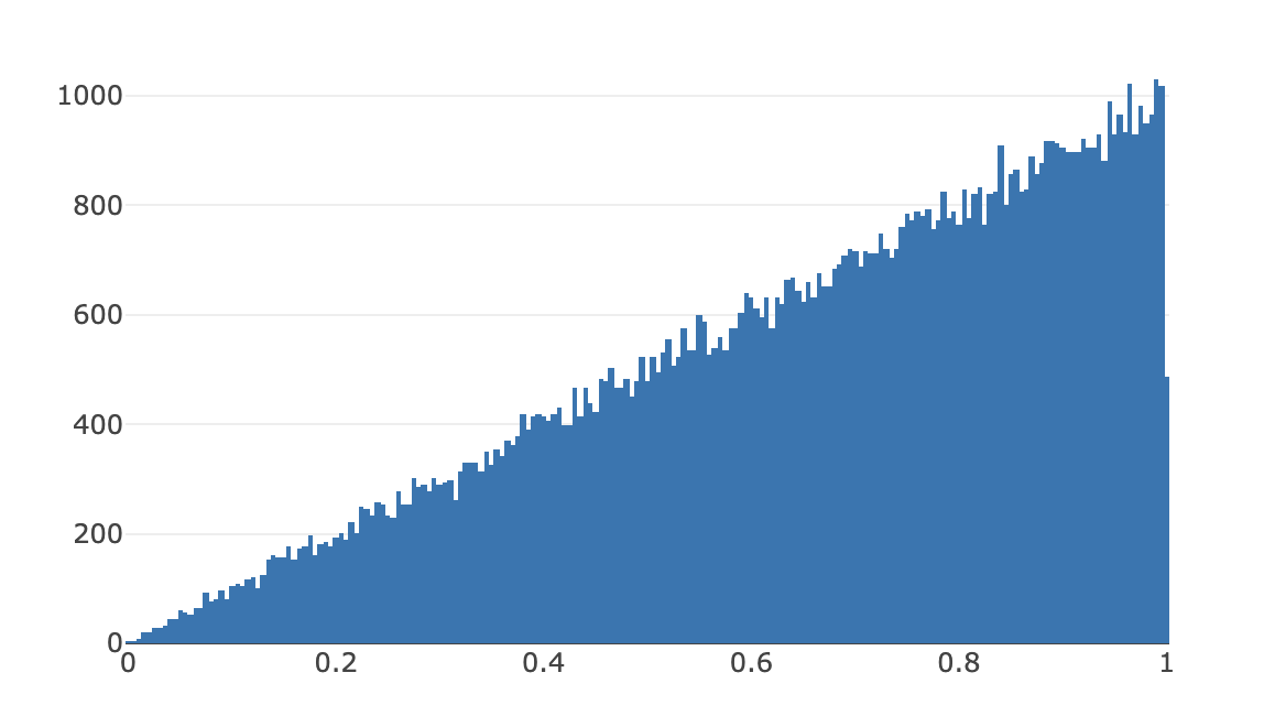
(This is the same as Math.pow(Math.random(), 1/2))

Interesting, but how do we get a normal distribution?

Getting a normal distribution

Combining the two above functions, we get closer. Their combination looks like an attempt at building a sandcastle with dry sand:

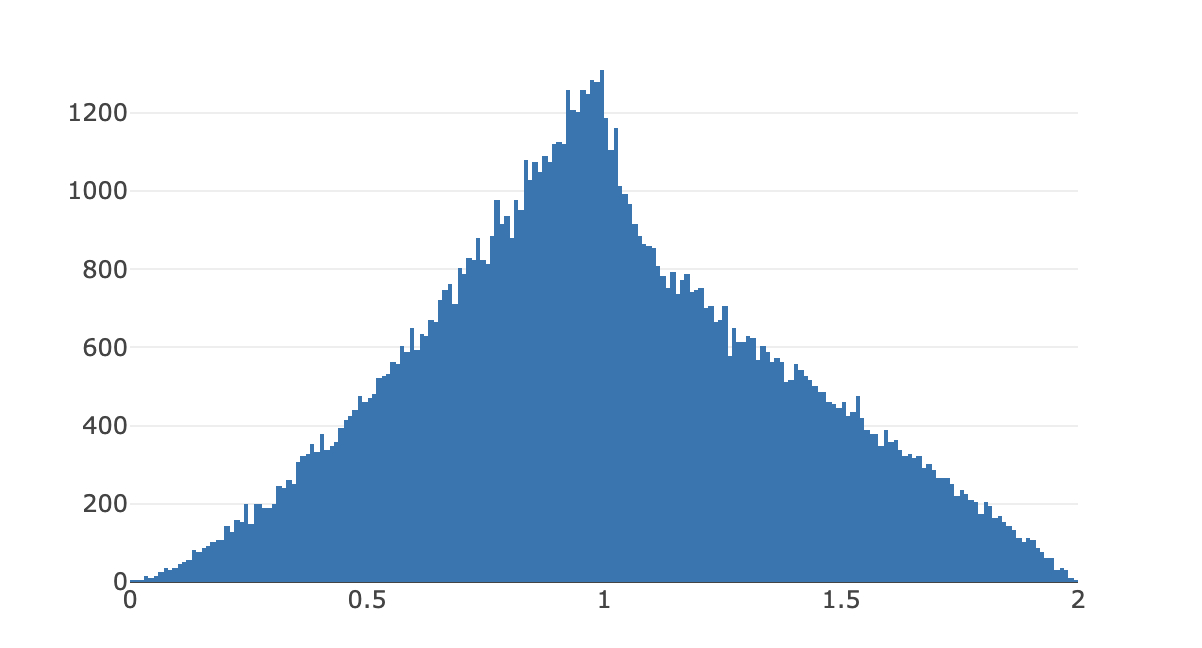
This distribution comes from Math.sqrt(Math.random()) + Math.pow(Math.random(), 2).

Remember the linear-looking Math.sqrt(Math.random()) function? When sampled three times and added together, it gives us a normal-looking distribution:

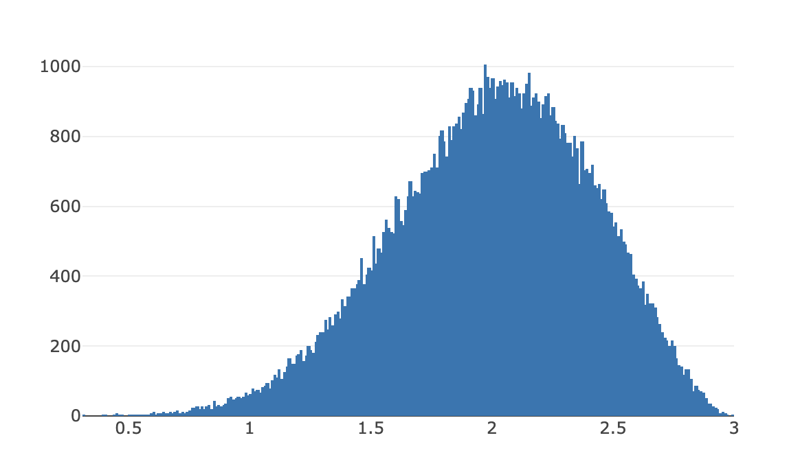
It's a little misshapen, but Math.sqrt(Math.random()) + Math.sqrt(Math.random()) + Math.sqrt(Math.random()) looks normal enough.

You might've guessed the pattern by now.

If we add Math.random() on itself a few times, we get an even-more normal looking distribution. The more times we do it, the more-normal the graph starts to look.

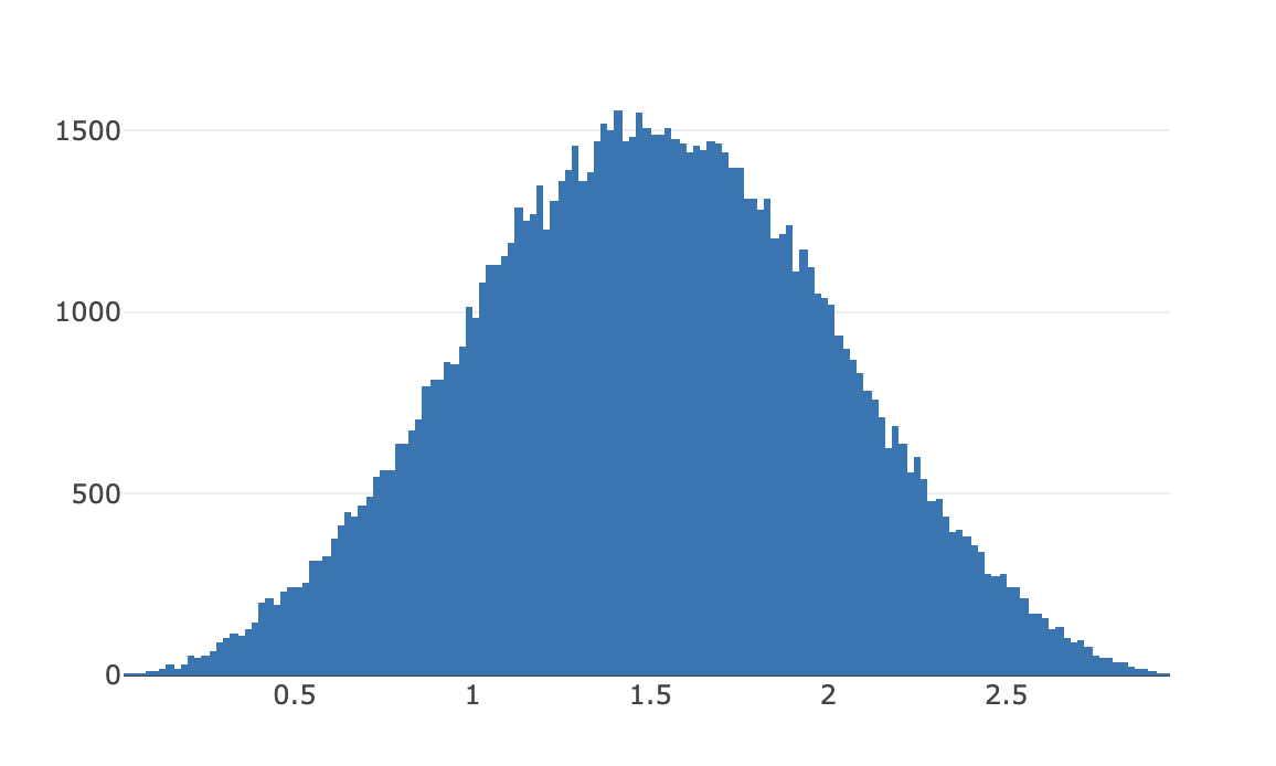
Math.random() + Math.random() + Math.random()

Great, but why does this work?

Why does adding samples of a uniform distribution give us a normal distribution?

This may seem confusing. So let's break down the possibilities. Imagine instead a uniform distribution that gives integers in the range [1, 6].

One provider of this distribution function is the common six-sided die.

When we have one die, we have an equal 1/6 chance of getting any value.

When we have two dice, each die still has an equal 1/6 chance of getting any value. However, if you've played any dice-rolling game, you might know that the chance of rolling a 12 is much lower than the chance of rolling a 7.

Why is this?

1. To roll a two, you must roll two 1's. We'll call this a (1, 1).
2. To roll a three, could roll:
   • (1, 2)
   • (2, 1)
3. To roll a four, you could roll:
   • (1, 3)
   • (2, 2)
   • (3, 1)
4. To roll a five, you could roll:
   • (1, 4)
   • (2, 3)
   • (3, 2)
   • (4, 1)
5. And so on, with permutation count increasing until 7, and then falling down after..
6. To roll an 11, you could roll:
   • (5, 6)
   • (6, 5)
7. And to roll a 12, you must roll a (6, 6).

Since each die roll is as likely as any other die value, each ordered die permutation (an ordered combination) is as likely as any other ordered die permutation.

That is, rolling a (1, 1) is as likely as rolling a (5, 6) (ordered). In the former, you have a 1/6 chance of rolling a 1, then another 1/6 of rolling the next one. In the latter, you have a 1/6 chance of rolling a five, then a 1/6 chance of rolling a 6.

That means that each permutation is equally likely, so the likelihood of rolling a specific sum is proportional to the number of permutations that can create it.

In other words, when you roll two dice, you have six ways to roll a 7, but only one way to roll a 2. Then, it would make sense that our distribution curve of combined dice values show 7 being six times as common as a 2.

The more dice you combine, the more you shift the distribution more closely to a normal distribution. Why does this approximate the normal curve shape specifically? It's explained by the central limit theorem, though honestly I don't quite understand it.

In lieu of that, here is a live demo I've created for you to simulate the probability of outcomes. It generates all possible sums of N rolls of an M-sided die, and plots the count of each sum:

Moving back to our real-world application, how can we create a bimodal distribution, with our normal probability distribution?

Creating a bimodal distribution

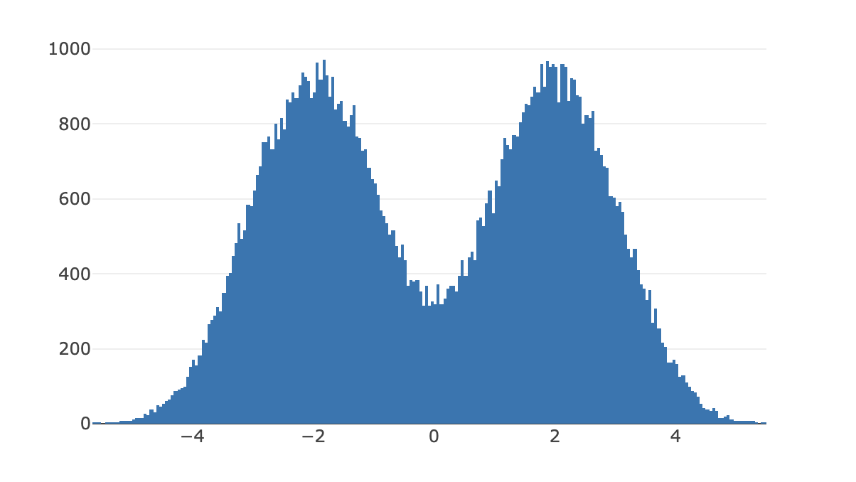
Well, the easiest way is to simply alternate between picking samples from two transformed normal probabilities:

// Where randNormal is a random-number-generating function
// with a normal probability distribution

const PEAK_DISTANCE = 0.7;
const PEAK_WEIGHT = 0.5;
function bimodalSample() {
	return Math.random() < PEAK_WEIGHT
		? randNormal(Math.random) * (1 - PEAK_DISTANCE)
		: randNormal(Math.random) * (1 - PEAK_DISTANCE) + PEAK_DISTANCE;
}

If this seems too easy, note that bimodal distributions are frequently caused by just this: sampling two different groups into the same dataset.

Sampling the above function gives us this plot.

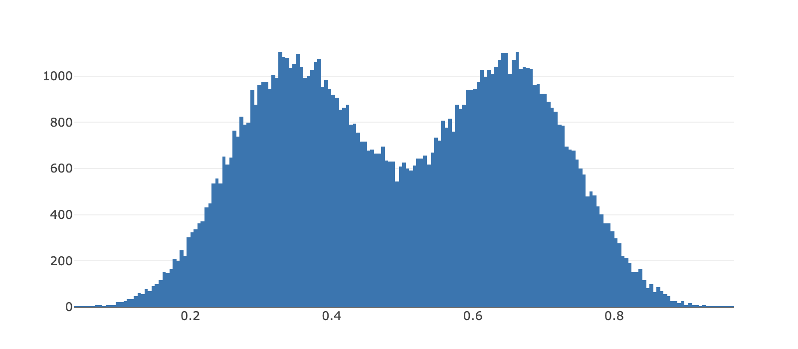
You can change the PEAK_DISTANCE and PEAK_WEIGHT parameters to change the distribution shape:

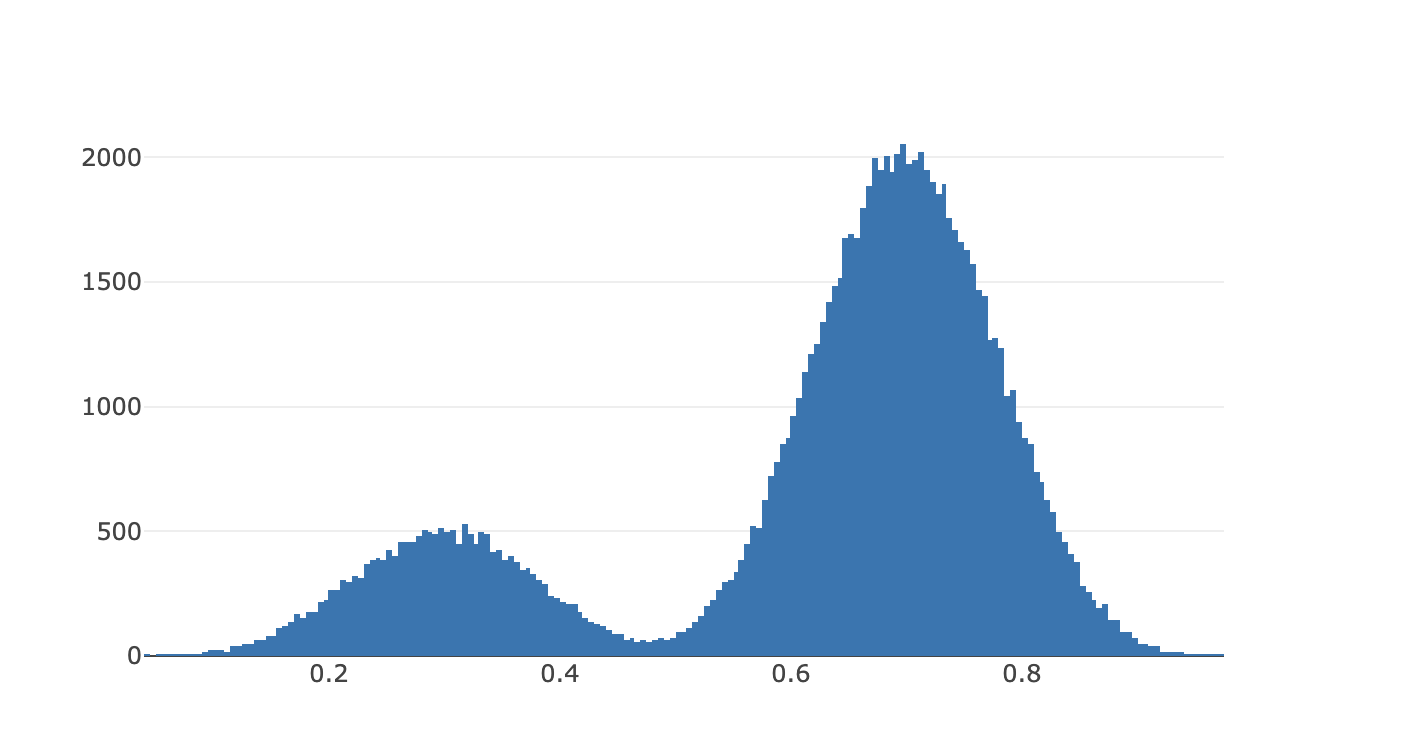
Here, we set PEAK_DISTANCE to 0.6, and PEAK_WEIGHT to 0.2.

For my use case, I kept the distribution even between the two sides. You can see its effects live on my blog homepage. Note that post angles won't change between updates or page refreshes. This consistency is achieved by using a Math.random()-like function which can be seeded with the post's ID. Seeding the function this way gives us the same angle for each post across refreshes.

And that's it! You now have a bimodal distribution using only a uniform distribution function as your randomness source.